Soptq

This article heavily references CSDN Backpropagation Algorithm (Process and Formula Derivation)

Basic Definitions#

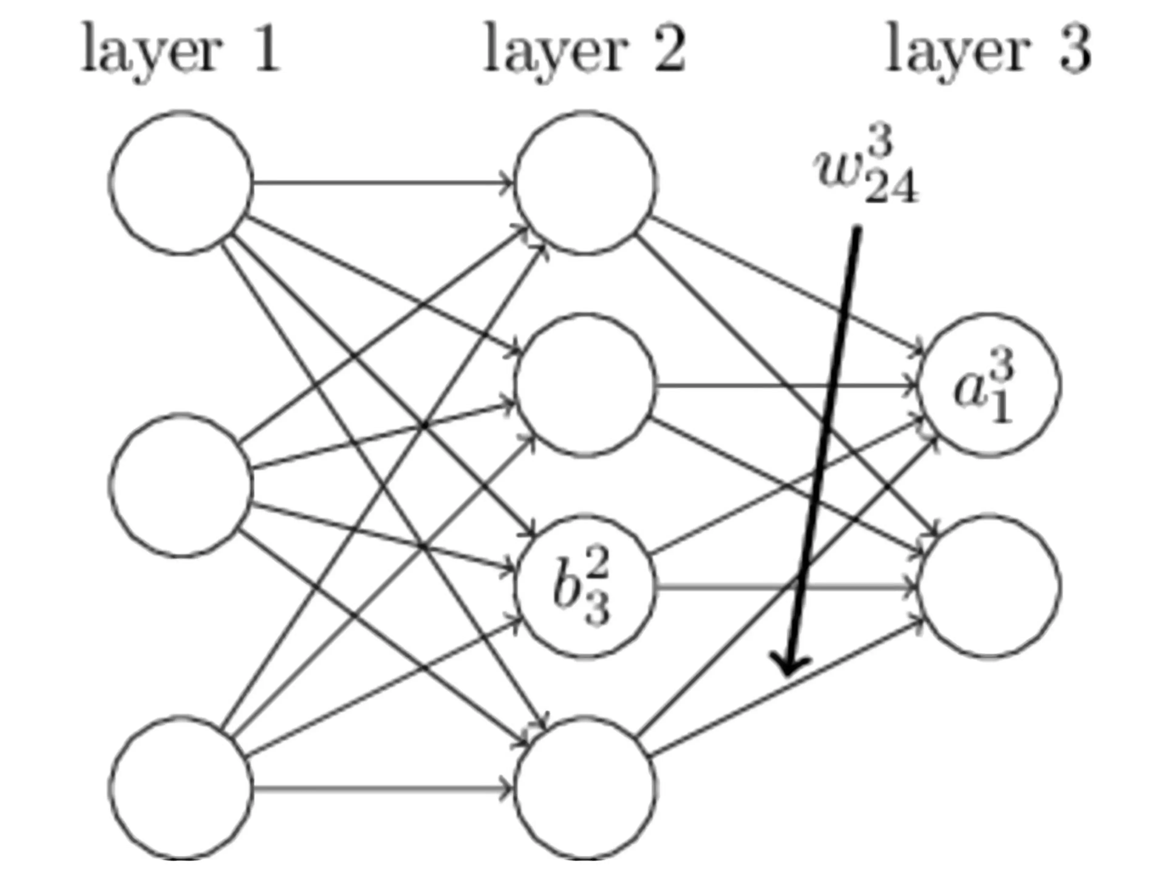
In the simple neural network shown in the above figure, layer 1 is the input layer, layer 2 is the hidden layer, and layer 3 is the output layer. We use the above figure to explain the meaning of some variable names:

Based on the above definitions, we can know that:

$z_{j}^{l} = \sum_{i}w_{ji}^{l}a_{i}^{l-1} + b_{j}^{l}$

$a_{j}^{l} = \sigma z_{j}^{l} = \sigma \left( \sum_{i}w_{ji}^{l}a_{i}^{l-1} + b_{j}^{l} \right)$

We define the loss function as the quadratic cost function:

$J = \frac{1}{2n} \sum_{x} \lvert \lvert y(x) - a^{L}(x) \rvert \rvert ^ {2}$

Where $x$ represents the input sample, $y(x)$ represents the actual classification, $a^{L}(x)$ represents the predicted classification, and $L$ represents the maximum number of layers in the network. When there is only one input sample, the loss function $J$ is denoted as:

$J = \frac{1}{2} \sum_{x} \lvert \lvert y(x) - a^{L}(x) \rvert \rvert ^ {2}$

Finally, we define the error generated in the $i$-th neuron in the $l$-th layer as:

$\delta_{i}^{l} \equiv \frac{\partial{J}}{\partial{z_{i}^{l}}}$

Formula Derivation#

The error generated by the loss function on the last layer of the neural network is:

$\begin{aligned}\delta_{i}^{L} &= \frac{\partial{J}}{\partial{z_{i}^{L}}}\\&=\frac{\partial{J}}{\partial{a_{i}^{L}}} \cdot \frac{\partial{a_{i}^{L}}}{\partial{z_{i}^{L}}}\\&=\nabla J(a_{i}^{L}) \sigma^{'}(z_{i}^{L})\end{aligned}$

$\delta^{L} = \nabla J(a^{L}) \odot \sigma^{'}(z^{L})$

The error generated by the loss function on the $j$-th layer of the network is:

$\begin{aligned}\delta_{j}^{l} &= \frac{\partial{J}}{\partial{z_{j}^{l}}} \\ &= \frac{\partial{J}}{\partial{a_{j}^{l}}} \cdot \frac{\partial{a_{j}^{l}}}{\partial{z_{j}^{l}}} \\ &= \sum_{i} \frac{\partial{J}}{\partial{z_{i}^{l+1}}} \cdot \frac{\partial{z_{i}^{l+1}}}{\partial{a_{j}^{l}}} \cdot \frac{\partial{a_{j}^{l}}}{\partial{z_{j}^{l}}} \\ &= \sum_{i} \delta_{i}^{l+1} \cdot \frac{\partial{w_{ij}^{l+1}a_{j}^{l} + b_{i}^{l+1}}}{\partial{a_{j}^{l}}} \cdot \sigma^{'}(z_{j}^{l}) \\ &=\sum_{i} \delta_{i}^{l+1} \cdot w_{ij}^{l+1} \cdot \sigma^{'}(z_{j}^{l}) \end{aligned}$

$\delta^{l} = \left( \left( w^{l+1} \right)^{T} \delta^{l+1} \right) \odot \sigma^{'}(z^{l})$

Therefore, we can calculate the gradient of the weights through the loss function:

$\begin{aligned} \frac{\partial{J}}{\partial{w_{ji}^{l}}} &= \frac{\partial{J}}{\partial{z_{j}^{l}}} \cdot \frac{\partial{z_{j}^{l}}}{\partial{w_{ji}^{l}}} \\ &= \delta_{j}^{l} \cdot \frac{\partial{\left( w_{ji}^{l}a_{i}^{l-1} + b_{j}^{l} \right)}}{\partial{w_{ji}^{l}}} \\ &= \delta_{j}^{l} \cdot a_{i}^{l-1} \end{aligned}$

$\frac{\partial{J}}{\partial{w_{ji}^{l}}} = \delta_{j}^{l} \cdot a_{i}^{l-1}$

Finally, we can calculate the gradient of the biases through the loss function:

$\begin{aligned} \frac{\partial{J}}{\partial{b_{j}^{l}}} &= \frac{\partial{J}}{\partial{z_{j}^{l}}} \cdot \frac{\partial{z_{j}^{l}}}{\partial{b_{j}^{l}}} \\ &= \delta_{j}^{l} \cdot \frac{\partial{w_{ji}^{l} a_{i}^{l-1} + b_{j}^{l}}}{\partial{b_{j}^{l}}} \\ &=\delta_{j}^{l} \end{aligned}$